How to Create Pivot Table in Excel?

Creating Pivot Tables in Excel can revolutionise how you analyse and interpret data. Whether you’re a Data Analyst, business professional, or student, knowing How to Create a Pivot Table in Excel is a valuable skill that can streamline your Data Analysis process.

So wait no more; t comprehensive blog will provide you insights on How to Create a Pivot Table in Excel and you will learn to leverage its powerful features to gain insights from your data. So, if you’re ready to unlock Excel's full potential for your Data Analysis needs, let’s dive into the world of Pivot Tables!

Table of Contents

1) What is a Pivot Table in Excel?

2) How to Create a Pivot Table in Excel? Six easy steps

3) How to refresh a Pivot Table in Excel?

4) How to move a Pivot Table to a new location?

5) Conclusion

What is a Pivot Table in Excel? 

To study trends based on your data, you can use a Pivot Table in Excel. It is a summary of your data wrapped in a chart. Pivot Table Excel interprets a lot of statistics on your screen. It enables you to group your data in many ways to reach fruitful conclusions more quickly.  

The "Pivot" in Pivot Table Excel refers to the ability to spin the data within the table to see it from various angles. So, when you perform a pivot, you are not increasing, decreasing, or altering your data. Instead, you are rearranging the data to make it easier to extract information that will be beneficial with the help of MS Excel Pivot Table. 

What is the use of Pivot Table in Excel?

Don't worry if you are still unsure what Pivot Tables are used for. It is one of those technologies that is much simpler to implement once you have a hold of it. 

The goal of Pivot Tables is to provide simple methods for quickly summarising vast volumes of data. They can be used to understand, present, or evaluate numerical data in depth and to find and respond to unpredicted questions more clearly. 

Here are seven situations where a Pivot Table acts as a solution:
 

How to Create a Pivot Table in Excel? Six easy steps

The following steps will help you understand How to Create a Pivot Table in Excel:

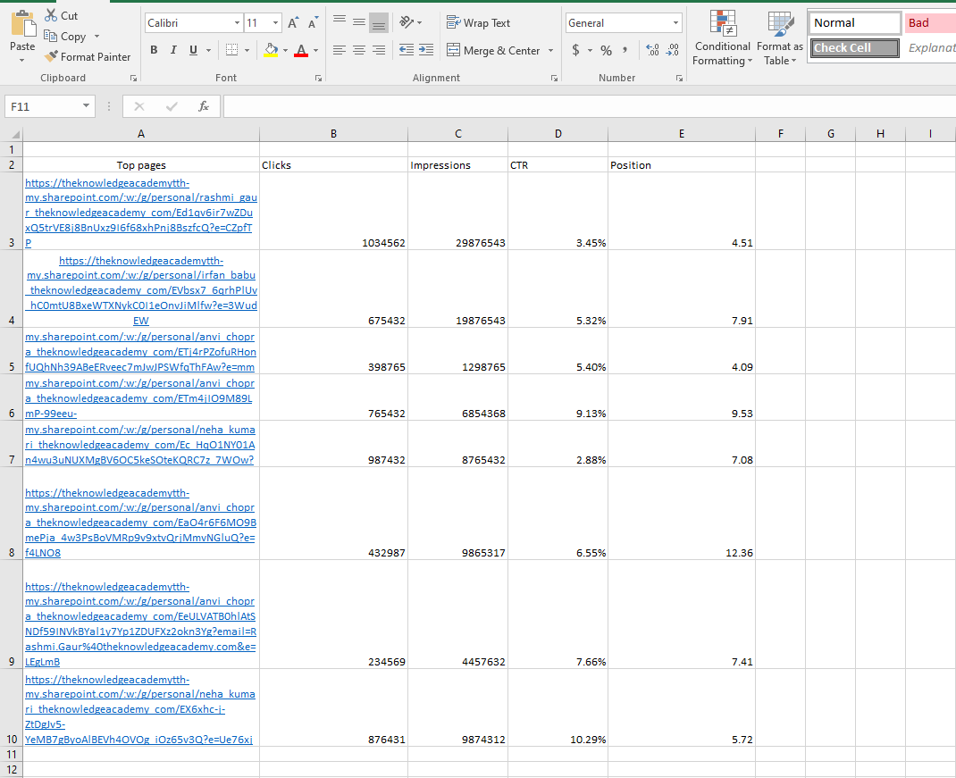
Step 1: Fill out a set of rows and columns with your data  

Every Pivot Table in Excel begins with a fundamental Excel table containing all your data. Enter your values into the designated rows and columns to build the table. Use the top row or column to group your values according to what they stand for.  

For example, if you want to create a table that records the blog post-performance data, you should have five columns that bring out the categorised data. Follow the steps below to understand the process.

Step 2: To make your Pivot Table, mark the cells 

After entering the data in your Excel spreadsheet, mark the cells you want to compile in a Pivot Table. Click on “Insert” and then select the “Pivot Table” icon. To make a Pivot Table, highlight the cells you want to use.

You may choose whether to launch this Pivot Table in a new worksheet or keep it in the current worksheet. Additionally, it will specify your cell range in the choice box. At the bottom of your Excel worksheet, you can navigate any newly opened sheets. After selection, click OK. 

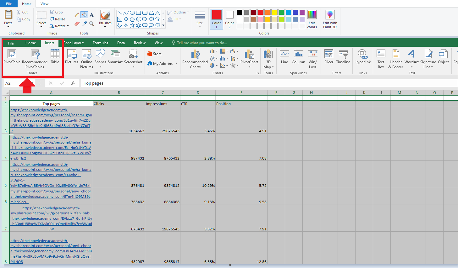
Note: If you are using the latest version of MS Excel, then the tables option under the “Insert” option, you will find a separate section of tables. Then, click on the “Tables” icon to select Pivot Table.

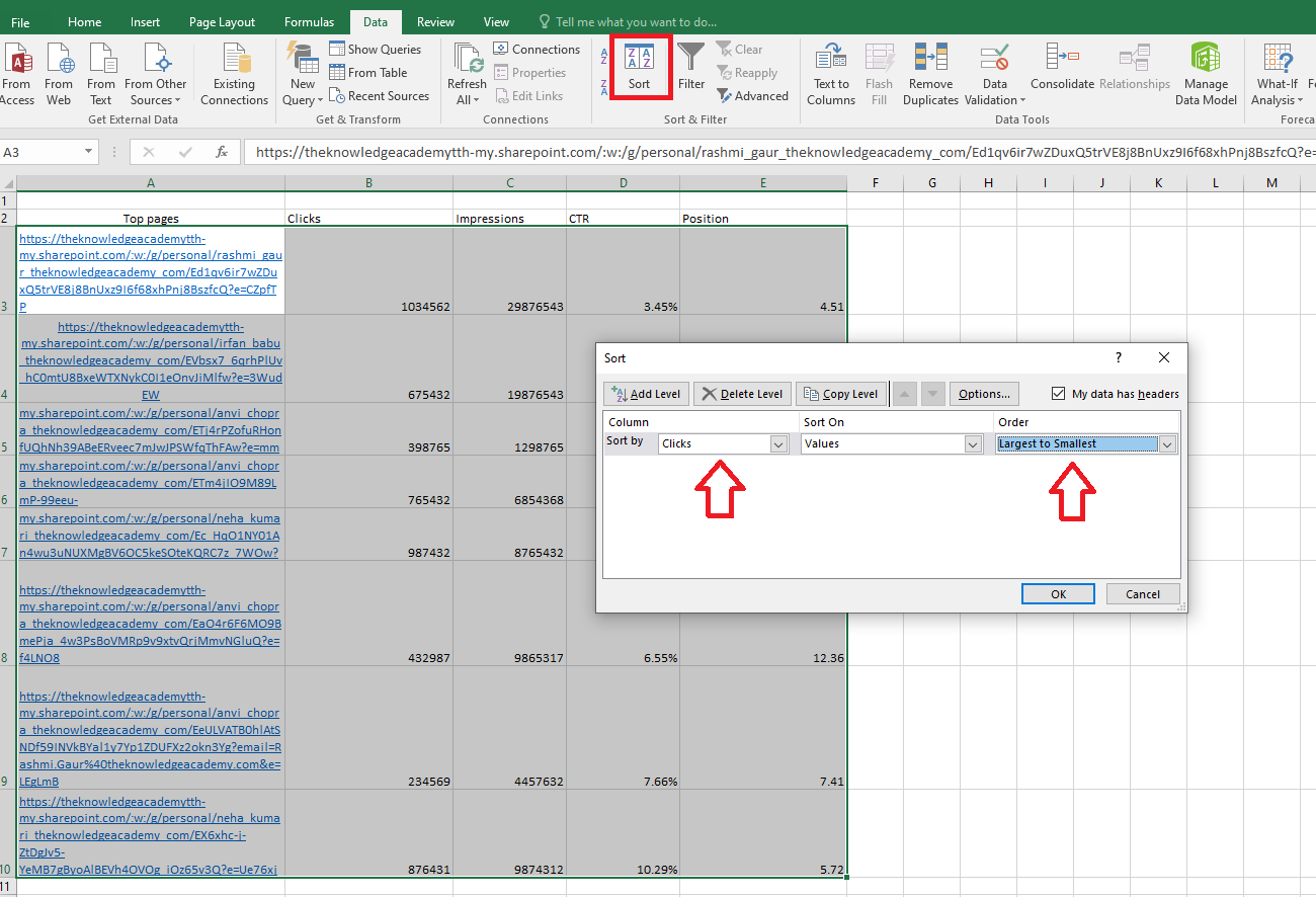
Step 3: Sort your data by a specific property

After creating the Pivot Table, right-click the values to be sorted in the data and select the sorting order you desire to use. This order can be ascending or descending in nature and is generally used for checking on a specific property within the Pivot Table.

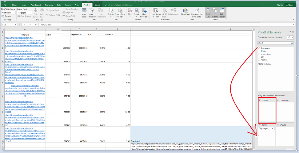
Step 4: Add a field by dragging it into the "Row Labels" section 

When Step 2 is finished, Excel will produce a blank Pivot Table for you. The next step is to drag and drop a field into the Row Labels section with a label that matches the names of the columns in your spreadsheet. By doing so, you can choose the specific identifier—blog post title, product name, etc.—by which the Pivot Table will arrange your data.

To organise blog data by post title, you must click and drag the “Top pages” field to the “Row Labels” area.

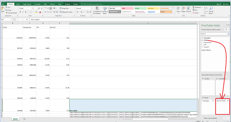
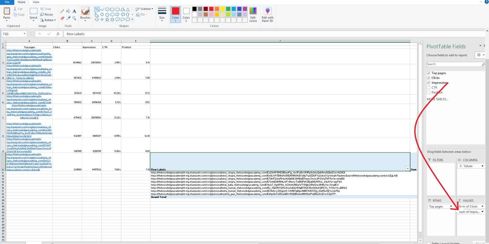
Step 5: Add a field by dragging it into the “Values Area” 

The next step is to add some values by dragging a field into the Values box once you have decided how to organise your data. 

Let's use the blogging data example again. So, if you want to sum up views of blog posts by title, drag the "Views" field into the Values box to achieve this. 

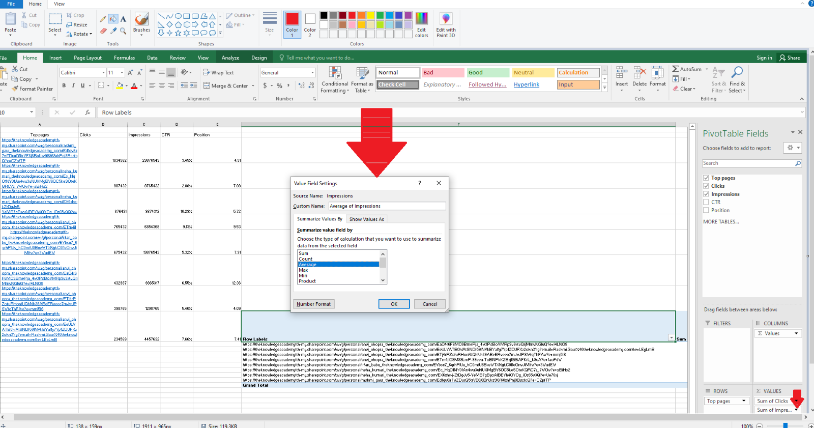
Step 6: Adjust your calculations as needed 

According to what you want to calculate, you can easily modify the default calculation to anything else, such as average, maximum, or minimum. 

Finally, you can adjust your calculations as per your requirements. Follow the steps in the succeeding images:

To access the menu, click on the tiny upside-down triangle next to your value and choose Value Field Settings. Follow the image below: 

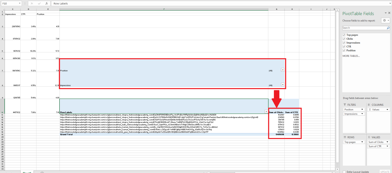
Drag and drop the fields into the value box and then to the filter box to find the actual position of the rows and columns. Follow the image below: 

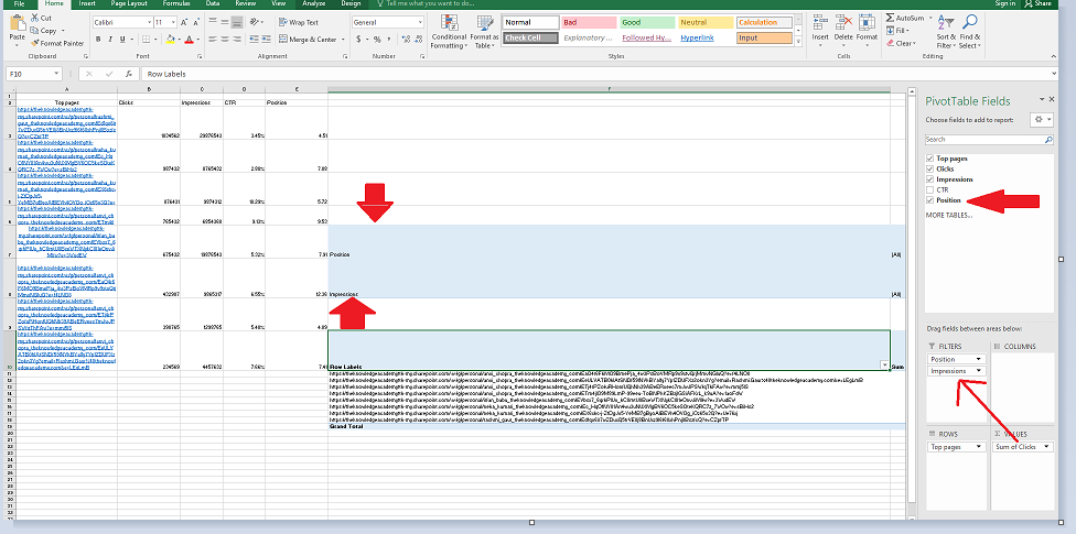
 Now, you can find the total of the sum of clicks, the sum of Click Through Rate (CTR), along with the position and impressions of the blog post. Follow the image below:

Finally, when you have categorised your data as per your requirement, save your work and use it as and when needed. The above steps will give you a clear idea of How to Create A Pivot Table in Excel.

Build your career as a Data Analyst. Check out our  Data Analysis Training Using MS Excel Course today!

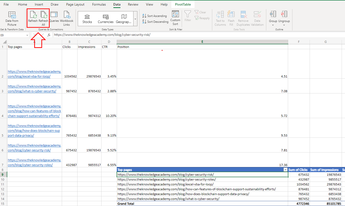
How to refresh a Pivot Table in Excel?

To refresh a Pivot Table on Excel, you can follow these steps:

1) Click on any cell within the Pivot Table.

2) Go to the “PivotTable” or “Data” ribbon on the menu.

3) Look for the “Refresh” or “Refresh All” button on the Data ribbon to refresh the data. Additionally, you can look for the “Refresh All” drop down menu on the PivotTable ribbon  which will also list “Refresh” pertaining to a single cell.

You can also set the Pivot Table to automatically refresh when you open the workbook at specific time intervals. To do this, go to the “PivotTable Options” or “Options” tab in the Excel ribbon. Under the “Data” tab, you’ll find the “Refresh data when opening the file” and “Refresh data every X minutes” options.
 

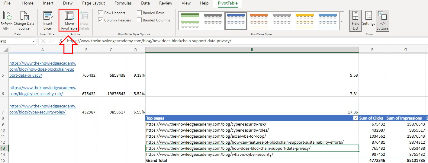
How to move a Pivot Table to a new location?

To move a Pivot Table on Excel to a different location, you can follow these steps:

1) Click on any cell within the Pivot Table to select it.

2) Go to the “PivotTable Analyze” or “Options” tab (depending on the Excel version), and select the “Move PivotTable” option.

3) In the “Move PivotTable” dialog box, select “New Worksheet” or “Existing Worksheet”, depending on where you want to move the Pivot Table to.

4) Click on the “OK” button to move the Pivot Table to the new location.

Note that when you move a Pivot Table, the data source and Pivot Table settings remain unchanged.
 

Conclusion 

The fundamentals of creating a Pivot Table have now been covered. We hope this blog gave you a detailed idea on How to Create a Pivot Table in Excel, the actions possible with the Pivot Table and find the solutions you are looking for.

To learn in detail to create advanced formulas, macros, and much more, you can sign up for our Microsoft Excel Expert MO201 Course now!