We may not have the course you’re looking for. If you enquire or give us a call on 01344203999 and speak to our training experts, we may still be able to help with your training requirements.
We ensure quality, budget-alignment, and timely delivery by our expert instructors.

Have you ever felt like you’re drowning in endless rows of data, searching for that one crucial piece of information? If that sounds familiar, it’s time to discover How to Use VLOOKUP in Excel- a tool that transforms data chaos into clarity.
Curious about unleashing this power? In this blog, you will learn How to Use VLOOKUP in Excel, including pro tips for using it across multiple workbooks. Ready to transform your data-handling game and impress your colleagues? Let’s dive into the world of VLOOKUP!
Table of Contents
1) What is VLOOKUP in Excel?
2) VLOOKUP Function
3) How to Use VLOOKUP in Excel?
4) How to do VLOOKUP in Excel with Two Spreadsheets?
5) How to do VLOOKUP in Excel with Two Workbooks?
6) Tips to Use VLOOKUP Function Efficiently
7) Conclusion
What is VLOOKUP in Excel?
VLOOKUP in Excel is a function that searches for a specified value in the first column of a table or range and returns a value from another column in the same row. It’s particularly useful for quickly retrieving data in large datasets, such as finding a product's price based on its ID.
The VLOOKUP function requires a lookup value and a table or range to search within. Additionally, you must specify the column number from which to retrieve the value. An optional argument is available to choose between an exact or approximate match. For more details on how VLOOKUP and similar functions are tested in interviews, check out our Excel Interview Questions guide.
VLOOKUP Function
The VLOOKUP Function is used to perform searches across columns in Excel spreadsheet. The total number of Functions in MS Excel is 504. and VLOOKUP function is one of those functions available in Lookup and reference type categories.
A VLOOKUP Function comprises four components necessary for building the VLOOKUP syntax.
|
=VLOOKUP(lookup_value, table_array, col_index_num, [range_lookup]) |
1) Look-up value: It is the value you wish to look up using this function.
2)The range: The lookup value must be placed within the first column in the range for VLOOKUP to work properly. Let's say the value you wish to look up is in cell A2; your range should start with A.
3) Column number: The third component of VLOOKUP is the column number within the range that contains the return value. For instance, if you specify the range as A5:D10, YOU NEED TO COUND A as the first column, B as the second, C as the third, and so on.
4) Approximation: An optional step where you can specify if you wish an approximate match or an exact match. It can be done with the help of “True” for an approximate match and “False” for an exact match. The default value for this component is “True” unless specified by the user.
The actual syntax of the VLOOKUP Function looks as follows after putting four components together: =VLOOKUP(lookup_value, table_array, col_index_num, [range_lookup])
The column with lookup data is always supposed to be on the left. The symbol of a semicolon (;) or comma (,) is used to separate the different parts of the Function.
Learn Microsoft Excel for Data Analysis with Data Analysis Training using MS Excel Training - build your career as a Data Analyst now!
How to Use VLOOKUP in Excel?
In Excel, take the steps in order to use VLOOKUP:
a) Identify your data: Ensure the data is structured in a table with the lookup values in the first column.
b) Select the cell: Choose the cell in which the result should be displayed.
c) Enter the formula: Type the VLOOKUP formula like this:
=VLOOKUP(lookup_value, table_array, col_index_num, [range_lookup])
d) Press Enter: The chosen cell will show the result.
How to do VLOOKUP in Excel with Two Spreadsheets?
Here’s how to do VLOOKUP in Excel with two spreadsheets, step by step:
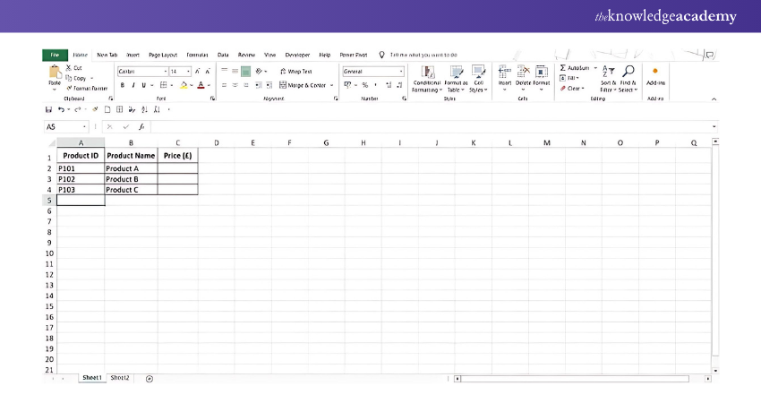
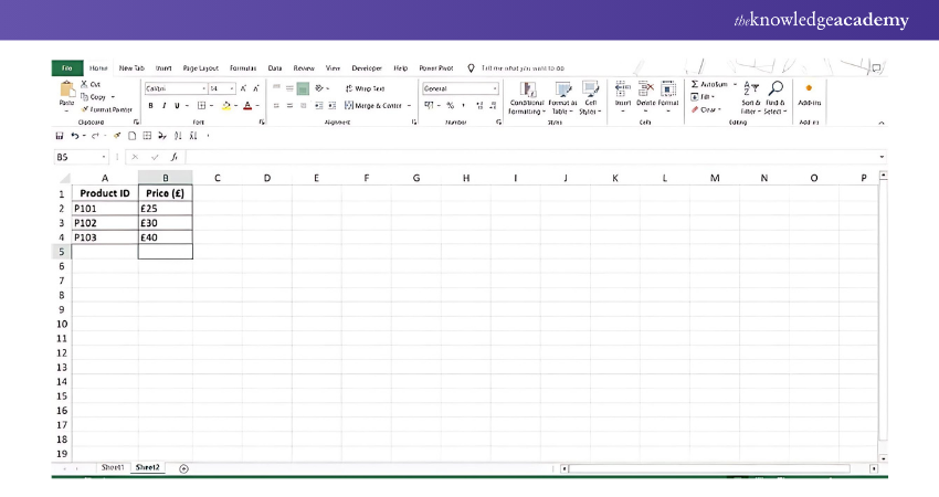
Step 1. Open Both Spreadsheets
Make sure both the source spreadsheet (with the data) and the destination spreadsheet (where you will apply the VLOOKUP) are open.
Step 2. Choose the Lookup Value
In the destination spreadsheet, select the cell where you want to display the result. Identify the lookup value that you will search for in the source spreadsheet (e.g., a product ID or name).
Step 3. Start the VLOOKUP Formula
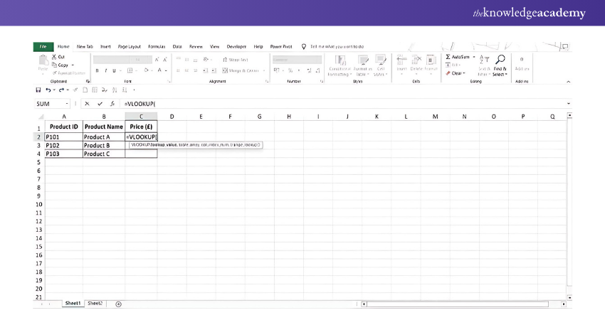
In the destination spreadsheet, select the cell where you want the result, and type:
|
=VLOOKUP( |
Step 4. Enter the Lookup Value
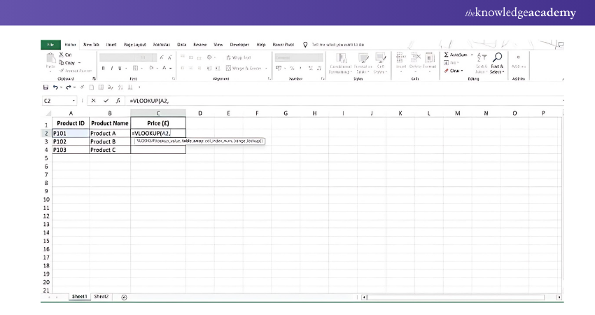
Next, enter the cell reference of the lookup value from the destination spreadsheet (e.g., A2). It will look like this:
|
=VLOOKUP(A2, |
Step 5. Select the Table from the Source Spreadsheet
a) Switch to the source spreadsheet, highlight the data range that contains the value you’re searching for and the column with the result.
b) Excel will automatically insert the file name, sheet name, and range into your formula like this:
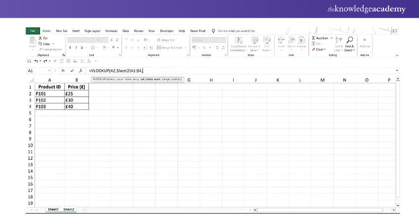
|
=VLOOKUP(A2, '[SourceSpreadsheet.xlsx]Sheet1'!A1:D100, |
Step 6. Specify the Column Index Number
Enter the column index number from the source spreadsheet where the value you want to return is located (e.g., 3 if it’s the third column).
It will look like this:
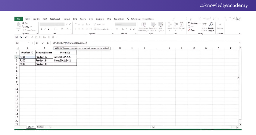
|
=VLOOKUP(A2, '[SourceSpreadsheet.xlsx]Sheet1'!A1:D100, 3, |
Step 7. Choose Exact or Approximate Match
Add FALSE or TRUE, depending on whether a match is exact or approximate, at the conclusion of the formula:
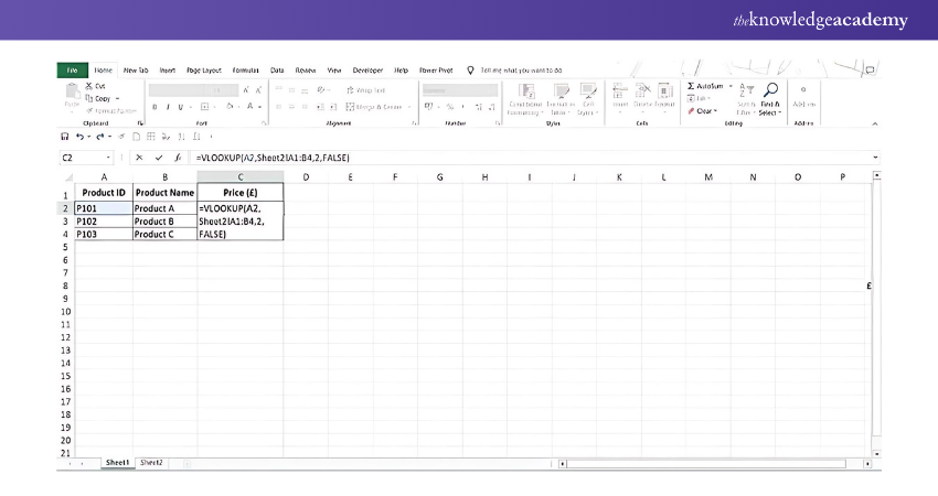
|
=VLOOKUP(A2, '[SourceSpreadsheet.xlsx]Sheet1'!A1:D100, 3, FALSE) |
Step 8. Press Enter
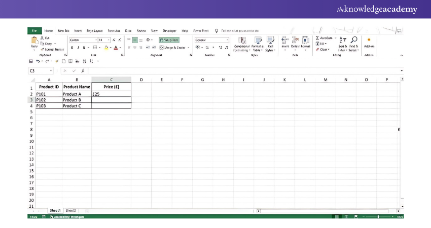
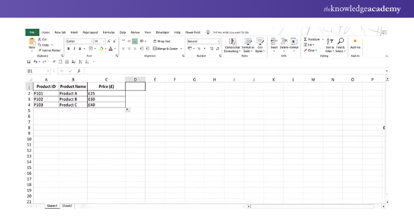
Press Enter, and Excel will pull the data from the source spreadsheet into the destination spreadsheet based on the lookup value.
Advance your business insights – sign up for the Business Analytics With Excel Course and become an analytics expert!
How to do VLOOKUP in Excel with Two Workbooks?
Here’s how to do a VLOOKUP in Excel with two workbooks, step by step:
Step 1. Open Both Workbooks
Open the workbook where you will apply the VLOOKUP and the workbook containing the data you want to search.
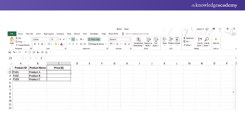
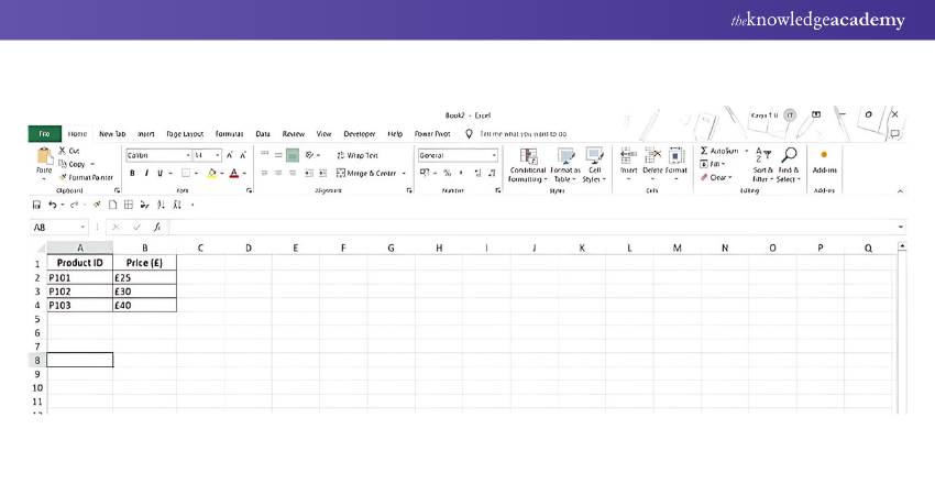
Step 2. Identify the Lookup Value
In the first workbook, choose the cell where you want to retrieve data. Also, determine the value you’ll be using to perform the lookup (e.g., a product ID).
Step 3. Start the VLOOKUP Formula
In the destination workbook, click on the cell where you want the result to appear and start typing the VLOOKUP formula:
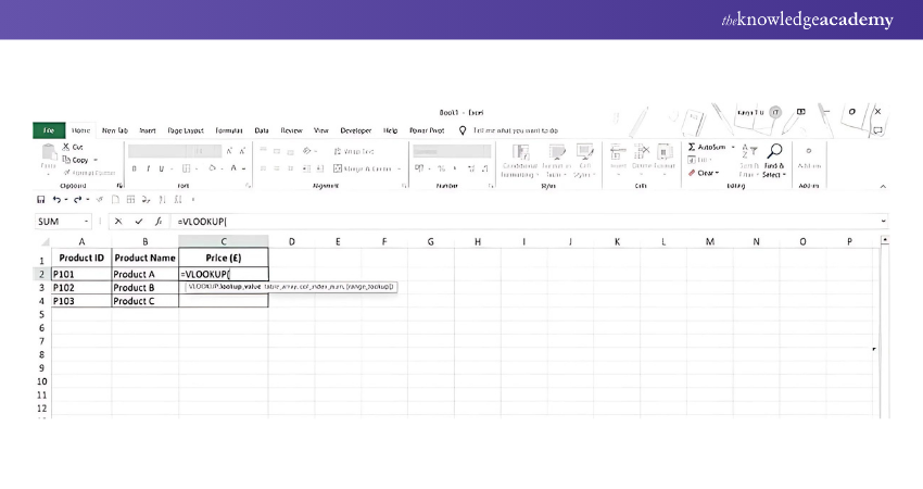
|
=VLOOKUP( |
Step 4. Enter the Lookup Value
Specify the lookup value by selecting the appropriate cell in the current workbook, for example:
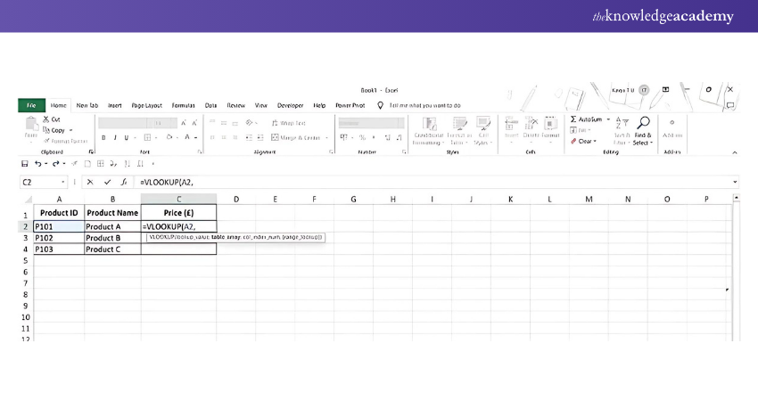
|
=VLOOKUP(A2, |
Step 5. Switch to the Source Workbook
Switch to the second workbook (where your data is located) and select the table or range of cells that includes both the lookup value and the data you want to retrieve.
Step 6. Highlight the Data Range
a) In the source workbook, highlight the range of cells that contains the lookup value (usually in the first column) and the column with the result.
b) Excel will automatically fill in the file name, sheet name, and cell range:
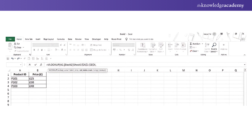
|
=VLOOKUP(A2, '[SourceWorkbook.xlsx]Sheet1'!A1:D100, |
Step 7. Enter the Column Index Number
Specify the column number (from the highlighted range) where you want to retrieve the value. For example, if the result is in the third column of your selected range:
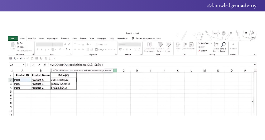
|
=VLOOKUP(A2, '[SourceWorkbook.xlsx]Sheet1'!A1:D100, 3, |
Step 8. Set Exact or Approximate Match
Depending on what you need, add TRUE for an approximate match or FALSE for a precise match:
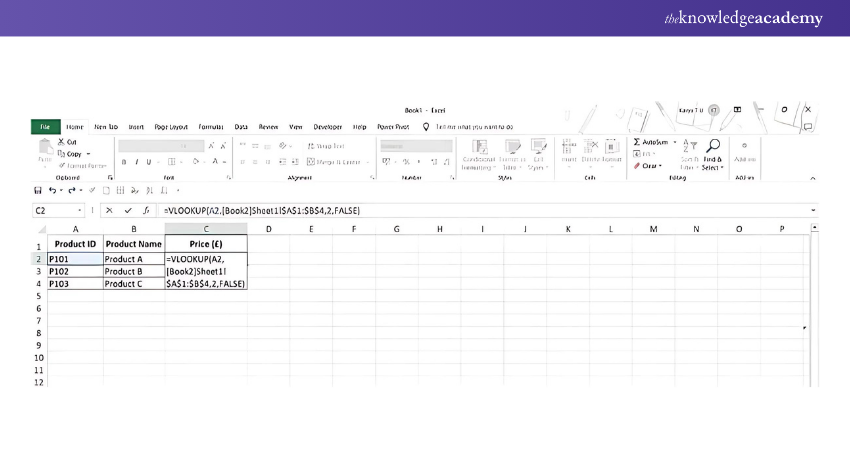
|
=VLOOKUP(A2, '[SourceWorkbook.xlsx]Sheet1'!A1:D100, 3, FALSE) |
Step 9. Press Enter
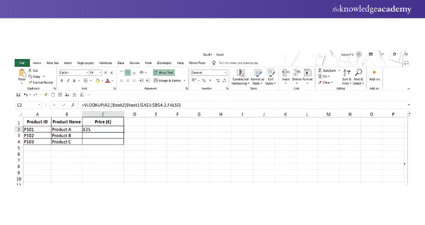
Press Enter, and Excel will return the result from the second workbook based on the VLOOKUP function.
Step 10. Save Both Workbooks
Ensure both workbooks are saved, as the formula will reference the second workbook for future calculations.
Enhance your Excel skills by learning Microsoft Excel VBA and Macro Training. Automate tasks and improve productivity now!
Tips to Use VLOOKUP Function Efficiently
Here are some tips to use the VLOOKUP function efficiently in Excel:
1) Use Absolute References for Table Ranges
When defining the table range, use absolute references (‘$A$1:$D$100’) to prevent the range from altering if you copy the formula to other cells.
2) Sort the Lookup Column (if using Approximate Match)
To obtain accurate results while using an approximate match ('TRUE'), sort the first column of your lookup range in ascending order.
3) Avoid Hardcoding Column Index
Instead of hardcoding the column index number, use the ‘MATCH’ function to make the formula more dynamic. Using MATCH Function allows automatic updates if columns are added or removed.
Example:
|
=VLOOKUP(A2, A1:D100, MATCH("Column Name", A1:D1, 0), FALSE) |
4) Use Named Ranges
Name your data ranges (e.g., ‘ProductList’) to make the formula easier to read and manage, especially if you have complex workbooks.
5) Utilise the IFERROR Function
To handle errors gracefully, wrap your VLOOKUP formula in an ‘IFERROR’ function. This ensures that when the lookup fails, you get a custom error message instead of ‘#N/A’.
Example:
| =IFERROR(VLOOKUP(A2, A1:D100, 3, FALSE), "Not Found") |
6) Use INDEX and MATCH as an Alternative
Consider using the ‘INDEX’ and ‘MATCH’ functions instead of VLOOKUP, especially when the lookup value isn't in the first column. This method is more flexible.
7) Avoid Large Data Ranges
Limit your table range to the smallest necessary size for better performance, particularly when working with large datasets.
8) Check for Exact Matches Carefully
When using ‘FALSE’ for an exact match, ensure that the data in your lookup column is free from extra spaces or formatting inconsistencies, as this could cause unexpected ‘#N/A’ errors.
9) Use Helper Columns for Complex Lookups
If your lookup involves multiple criteria, consider adding a helper column that concatenates values to create a unique key for VLOOKUP.
10) Save Processing Power
When using VLOOKUP on large datasets, use it sparingly and avoid overusing it in each cell. Try summarising data first or using it in specific areas.
Transform your accounting workflow with our Excel for Accounting Course - sign up now!
Conclusion
Mastering How to Use VLOOKUP in Excel opens a world of efficiency, turning daunting data searches into quick, seamless tasks. By using this powerful tool and avoiding common mistakes, you'll streamline your workflow, save time, and impress your team with your Excel expertise! Start applying VLOOKUP today to transform the way you handle data!
Learn how to create advanced formulas, macros and much more in our MS Excel training to become a Microsoft Excel Expert MO201 Training – join today!
Frequently Asked Questions
How to Compare Two Columns in Excel Using VLOOKUP?

To compare two columns in Excel using VLOOKUP, use the formula:
=IFERROR(VLOOKUP(A2, B:B, 1, FALSE), "Not Found")
This checks if values in column A exist in column B.
What are the Limitations of VLOOKUP in Excel?

VLOOKUP in Excel has limitations, including only searching left to right, requiring manual column index updates, being case-insensitive, being slow with large datasets, and lacking native support for multiple criteria. It also struggles with exact matches in large data.
What are the Other Resources and Offers Provided by The Knowledge Academy?

The Knowledge Academy takes global learning to new heights, offering over 3,000+ online courses across 490+ locations in 190+ countries. This expansive reach ensures accessibility and convenience for learners worldwide.
Alongside our diverse Online Course Catalogue, encompassing 17 major categories, we go the extra mile by providing a plethora of free educational Online Resources like Blogs, eBooks, Interview Questions and Videos. Tailoring learning experiences further, professionals can unlock greater value through a wide range of special discounts, seasonal deals, and Exclusive Offers.
What is The Knowledge Pass, and How Does it Work?

The Knowledge Academy’s Knowledge Pass, a prepaid voucher, adds another layer of flexibility, allowing course bookings over a 12-month period. Join us on a journey where education knows no bounds.
What are the Related Courses and Blogs Provided by The Knowledge Academy?

The Knowledge Academy offers Microsoft Excel Courses including Microsoft Excell, PowerPoint, Project Training. These courses cater to different skill levels, providing comprehensive insights into Create a Heat Map in Excel.
Our Office Application Blogs covers a range of topics related to Project Management Businesses, offering valuable resources, best practices, and industry insights. Whether you are a beginner or looking to advance your Microsoft Excel skills, The Knowledge Academy's diverse courses and informative blogs have you covered.

The Knowledge Academy is a world-leading provider of professional training courses, offering globally recognised qualifications across a wide range of subjects. With expert trainers, up-to-date course material, and flexible learning options, we aim to empower professionals and organisations to achieve their goals through continuous learning.

Upcoming Office Applications Resources Batches & Dates
Date
 Microsoft Excel Course
Mon 1st Jun 2026
Mon 6th Jul 2026
Mon 3rd Aug 2026
Tue 1st Sep 2026
Mon 5th Oct 2026
Mon 2nd Nov 2026
Mon 7th Dec 2026


 Top Rated Course


 If you wish to make any changes to your course, please


