How To Make Marksheet in Excel

You may have come across teachers and professors working hard, sweating and writing marks for each student in a register. But did you know where they lack after all this hard work? It is the smart work that can simplify making a Marksheet in Excel. 

Today, according to Acuity Training, one out of 25 professionals spend 80% of their time using Excel. So, it can work wonders for anyone who wants to use Excel and has become a one-stop solution for all your needs. 

So, if you are in the education sector, leave the hassle of marking everything on paper. Use Excel to effortlessly manipulate student data, all that while ensuring it is error-free. Wondering how to do it? Worry no more. 

In this blog, you will learn how to create a Mark Sheet in Excel step by step. You can create a complete, fully automated mark sheet management system in excel. 

Table of Contents 

1) What are the contents of Marksheet template in Excel? 

2) How to make Marksheet in Excel? 

3) What functions can be performed in a Marksheet in Excel? 

4) Benefits of creating Marksheet in Excel 

5) Conclusion

What are the contents of Marksheet template in Excel? 

One can completely eliminate the need for hard work by automating the process of creating mark sheets and report cards for students. Just use Marksheet in MS Excel. It provides various options to easily add, modify, sort, and remove data in the spreadsheet. 

Teachers can use step-by-step methods to create Marksheets and print report cards using MS Excel. Let’s take a detailed look at what these methods are: 

1) Basic data sheet

As the name suggests, it includes all the students’ essential information that needs to be printed on the report card. It can include: 

a) School name 

b) School address 

c) Academic Year detail 

d) Class teacher’s name 

e) Principal’s name 

f) Name of the student 

g) Class 

h) Division 

i) Roll number 

j) Total attendance 

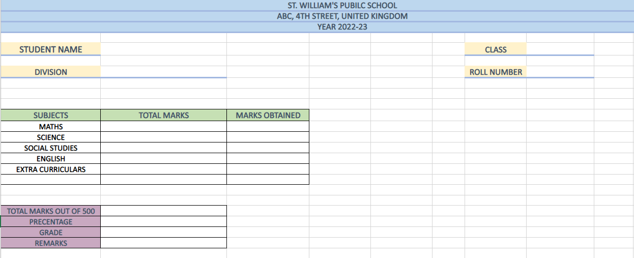
Here is an example of the Basic Information Sheet:

2) Template for grading system

The grading template essentially includes parameters by which the students’ marks can be divided, making it easy to calculate final grades. This also provides students and parents with insight into the grading system. You can create this sheet using the following steps:

In the above spreadsheet, you can see that marks are categorised based on grades. Further remarks are provided to explain the student’s performance throughout the academic year. 

3) Entering marks into the sheet

The last and vital step is to create a sheet with data values as students’ marks. You can enter data/marks in this sheet at your convenience. In simple terms, marks can be displayed on the spreadsheet in subject-wise, term-wise, and roll number-wise patterns.

This way you will create three sheets: 

1) Sheet1: To store the personal details 

2) Sheet2: To specify the grading system 

3) Sheet3: To insert the marks of each student 

Gain knowledge of the top 10 Excel Shortcuts with our Microsoft Excel Masterclass training course now! 

How to make Marksheet in Excel? 

After declaring all the necessary details, such as basic data of students and their marks, it is time to find the results of the students. To fulfil this purpose, you will need to perform various operations and enter formulas. This way, you will obtain a precise Marksheet format for your class, free of errors. 

But what are these operations? How do they work? Well, Microsoft Excel provides various formulas and functions to manipulate data. For example, in the Marksheet, if you want to add marks for Tracy, you can use the SUM() function, and you will get the total of all the marks within a few seconds. 

In the table below, we will find out the total marks, averages, grades, and the results of the students using various functions that MS Excel provides. 

Entering personal information 

The first step in creating a marksheet is to enter the personal details of the students. But the question arises, how do can you automate the process? Do you have to jump from one sheet to another? Well, the answer is no. Here, we will use the VLOOKUP() function to enter the basic information. So, let’s get started: 

Step 1: Firstly, enter the student’s roll number, class, and division in the specified columns. 

Step 2: Use the VLOOKUP function to enter the student’s name. Your marksheet will look as follows:


 

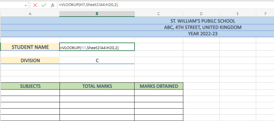
Here, in the VLOOKUP function, we first enter the lookup value, followed by a comma (H7,). The next step is to enter the sheet or array table from where we need to extract the data (Sheet2!A4:H20). Further, enter the column index number where you think the data lies.

Result: This way you will get the desired data value. For example, here we got Tracy as our data value. 

Additionally, if you also want to add other basic information like class teacher’s name, principal’s name, date of birth, or any other detail. You can use VLOOKUP and follow the similar format. 

Entering the marks obtained 

To insert the subject-wise marks of each student, you can again use the VLOOKUP() function, but with a twist. Here, you will need to apply conditional formatting to determine the performance of each student. Here’s how you can do it: 

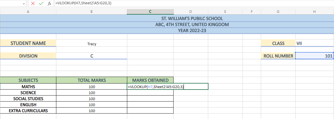
Step 1: Enter the VLOOKUP formula in the specified cell. Here for example, in the cell C12 where the total marks of Tracy will be extracted. The formula will be as follows: 

Step 2: Press Enter key. Then, to enter the same formula to find out the marks for other subjects, you just need to change the column index number according to the subject column in Sheet 1. This way you will get all the marks for Tracy, like this:

Conditional formatting

As you can see from the above image, finding the marks for Tracy has become easy. However, if you want to compare the marks, you can turn on conditional formatting in Excel. This way, teachers, students, as well as the parents will be able to see in which subjects does the student lack. Thus, providing an easy analysis of their marks. Just follow these steps to apply conditional formatting: 

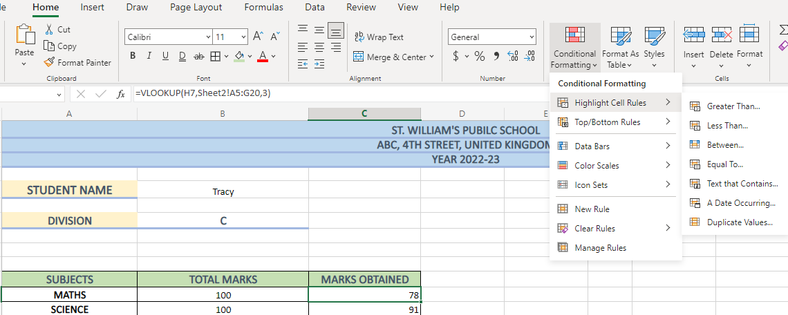
Step 1: 

a) Select the cells

b) Click on HOME ribbon 

c) Then click on CONDITIONAL FOMATTING option 

d) Go to HIGHLIGHT CELLS RULES 

e) Click LESS THAN


 

Step 2: Further, enter the minimum passing marks in the first box. 

Step 3: Select a colour of your choice from the dropdown box. This way you will be able to highlight the data values. 

Step 4: Click on OK button. 

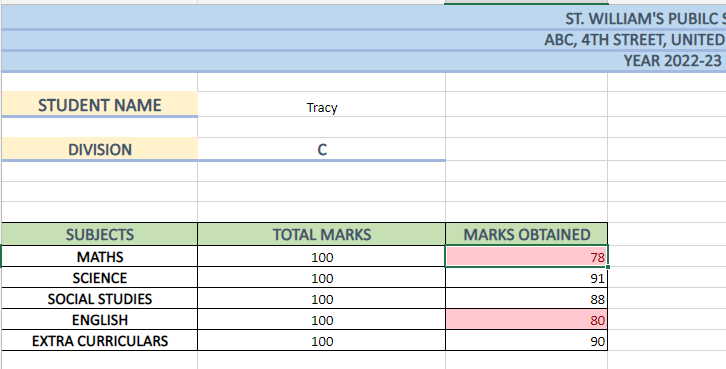
If student’s mark fails to meet the criteria set to pass, the data values will get highlighted in that colour. Your marksheet will look something like this:

Learn how to use Excel workbook settings and troubleshoot formulas with our Microsoft Excel Expert MO201 course now! 

Adding the marks

To determine the total marks of the students, you can use the SUM() function. Let's take a closer look at how this can be done: 

Simply insert the formula into the designated cell. The syntax for obtaining a total is as follows: 

a) Comma method: This method utilises comma(,) to insert each cell value. For example, SUM(A1,A2,A3,A4) 

b) Colon method: In this method, a colon replaces the comma, and you only need to specify the first and last cell values. For example, SUM(A1:A4)




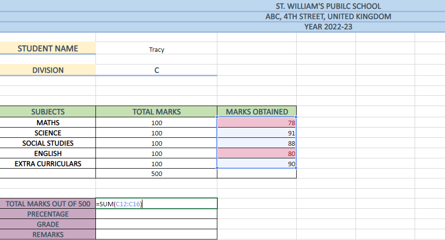
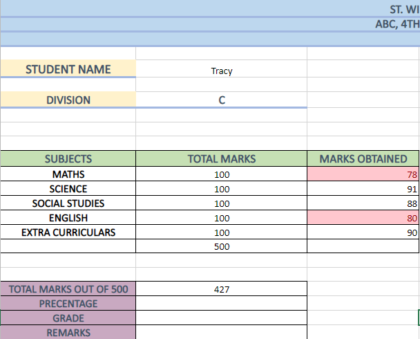
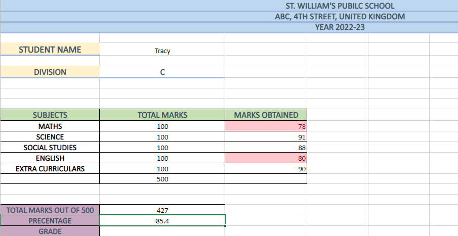
As a result, you will get the total marks for Tracy which is 427. 

Calculating the percentage

Calculating percentages is crucial to determine the final result of a student. For teachers, this process may be time-consuming and mentally taxing as it requires a lot of calculations. However, with Excel, this task becomes a breeze. You just need to follow the steps mentioned below: 

Step 1: Select the cell on which you want to apply the formula. 

Step 2: Enter the cell number that contains the total marks obtained by the student and divide it by the total marks, i.e., 500.



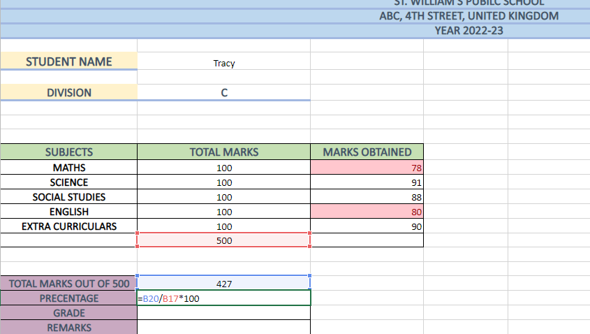
Result: You will get the percentage for Tracy by implementing a simple formula.

Finding student’s grade 

To find students’ grades, you can use IF() function. As we have already defined the criteria for marking percentages in Sheet 3, it will be easy to insert students’ grades in the Marksheet. Here is an example of how to declare the grades of the students using the IF() function: 

Step 1: First, enter all the possible parameters that can be applied to a cell range from Fig. 2. The table is referenced as the ”logical_test”. It contains the criteria of grading the percentages of the students. 

Step 2: Next, use logical operators such as “Greater Than,” “Less Than,” and “Equal To.” 

Step 3: Then compare the cell with the range where you want the grades to fit in. 

Result: As a result, you will get the grades that you previously specified for a range of percentages. 

By using the IF() function, you can determine if the percentage scored by the student is greater than or equal to 94, and the value will return as True. However, if the criteria are not met by the percentages, the argument will return as false. 

If you need to fulfil additional criteria and return True, you will need to write the IF function again. In this case, the IF function is applied 9 more times. 

Remember to close the bracket the same number of times s you have opened it, which in this case is nine times.



 

To insert the remarks 

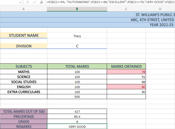
In order to add remarks for the students you can use the same function, i.e., the IF() function. Let's see how it works: 

Step 1: Insert the formula into the cell. 

Step2: Specify all the possibilities you want the remarks to fit in. Following is the manner you can do it:



Result: After you have specified the conditions, you will get your final remarks:

Benefits of creating Marksheet in Excel 

MS Excel can benefit you in many ways if you know how it use it efficiently. It not only helps teachers, but also provide a better understanding of the data to parents, giving a deep insight into students’ performance. But this is just one of the many benefits; some of the other benefits of Excel are as follows: 

1) Time-saving: Using formulas and functions in MS Excel makes calculations quick and easy, saving teachers time and effort. 

2) Reusable sheets: Unlike paper, a Marksheet in digital format can be altered multiple times and without any wastage. So, even if you need the Marksheet five or six times in a year, it will be easily accessible. 

3) Ready-to-view Marksheet: Excel allows users to print the Marksheets, making it easy to provide copies to students and parents. 

4) Improved data analysis: Excel presents data in a streamlined format, allowing teachers to compare students' performance and provide opportunities for improvement. 

Conclusion 

Creaking a Marksheet in Excel is quick and easy, and provides a better understanding of students’ marks. So, if you are an educator who is tired of writing and wasting time marking everything on paper, it’s time to switch to Microsoft Excel. 

Learn how to create pivot tables and charts, convert text and consolidate data in Excel with our Advanced Microsoft Excel 2019 55270AC course now!