Understanding Gradient Descent in Machine Learning Step by Step

Gradient Descent is one of the most important optimisation algorithms used in Machine Learning and Deep Learning. It helps models learn from data by minimising errors and improving prediction accuracy during the training process. Due to its effectiveness, it is widely used in neural networks, regression models, and other AI applications.

In this blog, you will explore Gradient Descent in Machine Learning, including its working process, types, advantages, and practical applications. It also explains how this optimisation technique improves model performance and supports the development of efficient AI-driven solutions.

Table of Contents

1) What is Gradient Descent in Machine Learning?

2) How does Gradient Descent in Machine Learning Work?

3) Types of Gradient Descent in Machine Learning

4) Challenges and Limitations of Gradient Descent in Machine Learning

5) Tips for Tuning Gradient Descent in Machine Learning

6) Conclusion

What is Gradient Descent in Machine Learning?

Gradient Descent is one of the most important optimisation Techniques in Machine Learning. It plays a pivotal role in making accurate data-based predictions by training Machine Learning Methods. At its core, Gradient Descent is an iterative algorithm used to minimise a cost function. The cost function measures the disparity between the predictions made by a model and the actual data.

The goal of Gradient Descent in Machine Learning is to find the set of model parameters that result in the lowest possible value of the cost function, indicating the best fit of the model to the data. Here's a simplified breakdown of how the Gradient Descent Algorithm works:

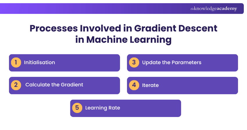
1) Initialisation: The process begins with an initial guess for the Machine Learning model's parameters. These parameters, which may include weights and biases, are essential for making predictions.

2) Calculate the Gradient: Next, the Machine Learning Algorithm computes the gradient of the cost function concerning the model's parameters. The gradient is a vector that is aligned in the direction of the steepest increase in the cost function.

3) Update the Parameters: The Machine Learning Algorithm then adjusts the model's parameters in the opposite direction of the gradient. This adjustment is controlled by a hyperparameter called the learning rate, which determines the size of each step.

4) Iterate: Steps 2 and 3 are repeated multiple times, with the Machine Learning model's parameters being updated in each iteration. The algorithm continues to adjust the parameters until it reaches a point where further changes don't significantly reduce the cost function. This signifies the algorithm has converged, and the parameters are optimised.

5) Learning Rate: The learning rate is a crucial factor in the process. If it's too small, the algorithm may converge very slowly. If it's too large, it may overshoot the minimum of the cost function and potentially diverge. Selecting an appropriate learning rate often involves experimentation and fine-tuning.

Gradient Descent is like navigating a landscape, where the cost function represents the terrain, and the goal is to find the lowest point. The algorithm starts at an initial position, calculates the direction of the steepest descent (indicated by the gradient), and takes steps in that direction. This iterative process continues until the algorithm reaches a point where further adjustments to the parameters have a negligible impact on the cost function.

Overall, Gradient Descent is a foundational technique that underpins the training of various Machine Learning Models like linear regression, neural networks, and deep learning architectures. It allows models to adapt and learn from data, making them more accurate and effective in making predictions.

Learn to build intelligent models, analyse data, and solve real-world problems using Machine Learning techniques with our Machine Learning Training- Join today!

How does Gradient Descent in Machine Learning Work?

Imagine Gradient Descent in Machine Learning as a hiker trying to find the lowest point in a valley. The hiker starts at an initial position (a), and the goal is to reach the lowest point (b) on the valley floor. In the context of Machine Learning, this valley represents the cost function, and the hiker is the optimisation algorithm.

The algorithm's objective is to minimise the cost function, and it does so by moving in the direction of the steepest descent, which is indicated by the gradient of the cost function (Δf(a)). Here's an example of Gradient Descent Machine Learning Algorithm:

The hiker (algorithm) starts at a random point on the cost function (valley) and takes one step at a time in the steepest downward direction (from the top to the bottom of the valley). The process continues until the algorithm reaches the point where the cost function is minimised.

In the context of Machine Learning, this process is applied to adjust model parameters, such as weights and biases, to minimise the cost function. The goal is to find the values of these parameters that correspond to the minimum of the cost function, resulting in a model that makes accurate predictions.

Gradient Descent is a key optimisation algorithm in Machine Learning, and its effectiveness relies on carefully choosing the learning rate and iteratively updating the model's parameters to reach a minimum point on the cost function.

Build practical skills to analyse data and create smarter insights using AI and Machine Learning with our AI and ML with Excel Training Course - Join now!

Types of Gradient Descent in Machine Learning

In the realm of Machine Learning (ML) optimisation, Gradient Descent comes in various flavours, each catering to specific scenarios and requirements. The primary types of Gradient Descent in Machine Learning Algorithms are as follows

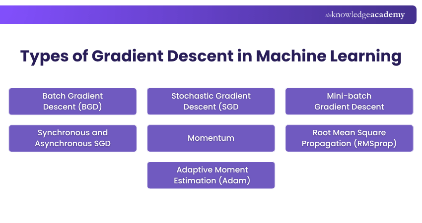
1) Batch Gradient Descent (BGD): BGD is the classical form of Gradient Descent, where the entire training dataset is used to calculate the gradient of the cost function in each iteration. It provides a precise estimate of the gradient but can be computationally expensive, especially with large datasets. BGD guarantees convergence to a minimum but might be slower for massive datasets.

2) Stochastic Gradient Descent (SGD): SGD takes a different approach by randomly selecting a single data point from the training set in each iteration to calculate the gradient. It is computationally more efficient and can lead to faster convergence, especially in large datasets. However, the randomness in selecting data points introduces noise in the optimisation process, which can cause oscillations in the cost function. Despite this noise, SGD is effective and widely used.

3) Mini-batch Gradient Descent: Mini-batch Gradient Descent strikes a balance between BGD and SGD. Instead of using the entire dataset or just one data point, mini-batch Gradient Descent divides the training dataset into small, equally sized batches. In each iteration, it computes the gradient using one of these batches. It combines the advantages of both BGD and SGD, offering a good compromise between accuracy and efficiency. It is the most commonly used variant in practice, especially in deep learning.

4) Synchronous and Asynchronous SGD: In parallel computing environments, synchronous SGD involves multiple workers updating the model parameters together based on a shared gradient calculation. Asynchronous SGD, on the other hand, allows workers to update parameters independently. While synchronous SGD ensures consistent updates and convergence, it can suffer from slower training times due to synchronisation. Asynchronous SGD can be faster but may lead to parameter inconsistencies.

5) Momentum: Momentum is an enhancement to standard Gradient Descent that helps accelerate convergence, especially when the cost function is poorly conditioned or contains high-curvature areas. It adds a momentum term to the parameter updates, which allows the algorithm to accumulate velocity in the direction of the gradient. This momentum helps the algorithm traverse shallow local minima and reach the global minimum more efficiently.

6) Root Mean Square Propagation (RMSprop): RMSprop is an adaptive learning rate optimisation algorithm that adjusts the learning rate for each parameter. It calculates the exponentially weighted moving average of past squared gradients for each parameter. This helps handle issues with varying gradient magnitudes and speeds up convergence.

7) Adaptive Moment Estimation (Adam): Adam is another adaptive learning rate optimisation algorithm that combines the benefits of momentum and RMSprop. It maintains moving averages of both past gradients and their squared values, adjusting the learning rate for each parameter. Adam is widely used in deep learning and is known for its efficient convergence.

These variants and enhancements to Gradient Descent cater to different Machine Learning scenarios, allowing practitioners to pick the most suitable approach based on the specific dataset and optimisation goals. Mini-batch Gradient Descent, in particular, is a popular choice in many deep learning applications, as it offers a balance between accuracy and efficiency.

Challenges and Limitations of Gradient Descent in Machine Learning

While Gradient Descent is a powerful optimisation algorithm that underpins many Machine Learning techniques, it is not without its challenges and limitations. Understanding these issues is crucial for effectively applying Gradient Descent in real-world scenarios. So, let's take a look at the Challenges of Gradient Descent in Machine Learning:

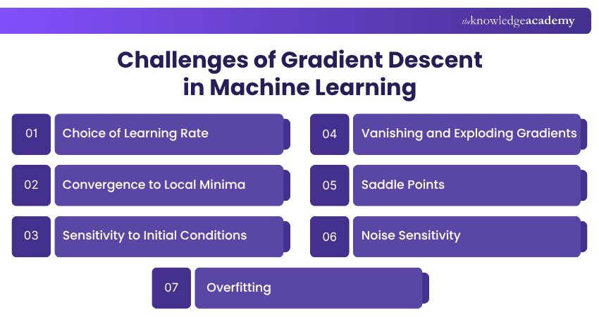
1) Choice of Learning Rate: Selecting an appropriate learning rate is a critical challenge. A learning rate that is considered too small can lead to slow convergence, while one that is too large may cause divergence. Hyperparameter tuning is often required to find the right learning rate for a specific problem, which can be a time-consuming process.

2) Convergence to Local Minima: Gradient Descent is not guaranteed to find the global minimum of the cost function, especially in complex, high-dimensional spaces. It may converge to local minima, which are suboptimal solutions. Techniques like random initialisation and using advanced optimisation algorithms can mitigate this issue.

3) Sensitivity to Initial Conditions: The choice of initial parameter values can significantly impact the optimisation process. Starting from different initial points can lead to different solutions. This sensitivity requires careful initialisation strategies, such as Xavier/Glorot initialisation for deep neural networks.

4) Vanishing and Exploding Gradients: In deep learning, as gradients are backpropagated through many layers, they can become vanishingly small or explosively large. Vanishing gradients can cause slow training while exploding gradients can lead to numerical instability. Techniques like using activation functions with non-zero gradients and gradient clipping are used to address these problems.

5) Saddle Points: Gradient Descent can stall at saddle points, which are points where the gradient is zero but not a minimum. This can slow down convergence as the algorithm lingers at such points. Advanced optimisation algorithms like momentum and stochastic Gradient Descent with mini-batches help navigate saddle points more effectively.

6) Noise Sensitivity: In stochastic Gradient Descent (SGD), the use of randomly selected data points introduces noise in the optimisation process. This noise can lead to oscillations in the cost function and hinder convergence. Techniques like learning rate schedules and adaptive learning rates (e.g., Adam) can help stabilise the training process in SGD.

7) Overfitting: Gradient Descent can make the model overfit the training data, especially when the model is too complex or the dataset is small. Regularisation techniques like L1 and L2 regularisation, are used to prevent overfitting by adding penalty terms to the cost function.

Understanding these challenges and limitations is essential for practitioners to effectively apply Gradient Descent in Machine Learning. In many cases, combining Gradient Descent with advanced optimisation techniques and regularisation methods can help overcome these issues and achieve better model performance.

Gain practical expertise in neural networks and AI-driven model development with our Neural Networks with Deep Learning Training – Register now!

Tips for Tuning Gradient Descent in Machine Learning

Tuning Gradient Descent is a crucial aspect of optimising Machine Learning Models. Achieving the right balance of hyperparameters and settings can greatly impact the effectiveness as well as the efficiency of the optimisation process. Here are some essential tips for tuning Gradient Descent:

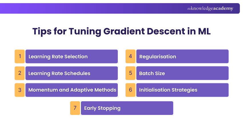
1) Learning Rate Selection: Carefully choose the learning rate, as it's a fundamental hyperparameter. Start with a moderate learning rate and experiment with values both smaller and larger to find the best fit for your specific problem. Learning rate schedules, such as learning rate decay, can also be beneficial.

2) Learning Rate Schedules: Implement learning rate schedules that adapt the learning rate during training. These schedules can help maintain stability during optimisation. Common schedules include step decay, exponential decay, and the Cyclical Learning Rate policy.

3) Momentum and Adaptive Methods: Consider using momentum or adaptive optimisation methods like RMSprop and Adam. These methods can help overcome issues like vanishing gradients and speed up convergence.

4) Regularisation: Apply regularisation techniques like L1 and L2 regularisation to prevent overfitting. These techniques add penalty terms to the cost function to encourage simpler models.

5) Batch Size: Experiment with different batch sizes in mini-batch Gradient Descent. Smaller batches can introduce more noise but may help escape local minima, while larger batches may provide more stable updates.

6) Initialisation Strategies: Use appropriate initialisation strategies for model parameters, such as Xavier/Glorot initialisation for deep neural networks. Careful initialisation can help mitigate sensitivity to initial conditions.

7) Early Stopping: Implement early stopping to prevent overfitting and save training time. Monitor the validation performance and stop training when it no longer improves.

Tuning Gradient Descent in Machine Learning requires a combination of domain knowledge, experimentation, and a deep understanding of the problem at hand. By employing these tips, you can fine-tune Gradient Descent to achieve optimal model performance and efficient training.

Conclusion

Gradient Descent is a fundamental optimisation algorithm that plays a vital role in training Machine Learning and Deep Learning models efficiently. Understanding its working process, types, challenges, and tuning techniques helps improve model accuracy and performance. With proper optimisation strategies, Gradient Descent enables the development of intelligent and reliable AI-driven solutions across various applications.

Enhance automation, monitoring, and operational efficiency using AI-driven DevOps practices with our Artificial Intelligence (AI) for DevOps Course – Sign in now!