How to use the MATCH function in Excel with formula examples

Wondering How to Use the Match Function in Excel? The “MATCH” function is a powerful and versatile tool that helps analysts find the position of a value in a range of cells. The best part about this function is that it can be combined with several other functions, such as INDEX, VLOOKUP, or HLOOKUP, to perform intricate tasks seamlessly. Continue diving into this blog to study the “MATCH” function in-depth and how you can utilise it to ensure seamless working for data professionals. Let’s get the wheels rolling!

Table of Contents

1) What is the “MATCH” Function in Excel?

2) How to Use "MATCH" Function in Excel?

3) MATCH Function in Excel - Key pointers

4) Conclusion

What is the “MATCH” Function in Excel?

The MATCH function is a built-in lookup and reference tool in Excel that returns the position of a specific value within a row, column, or array. Rather than returning the value itself, it shows where the value is located in the range.

For example, if the range A2:A5 contains the values 2, 4, 6, and 8, and you search for 4 using the formula =MATCH(4, A2:A5, 0), the result will be 2, as 4 is the second value in that range.

Uses of the MATCH Function:

1) Commonly combined with the INDEX function to locate values dynamically in rows or columns.

2) Helps find exact or approximate positions based on the match type.

3) Can enhance VLOOKUP by dynamically referencing column positions.

MATCH Function Syntax

a) lookup_value – the value you want to find

b) lookup_array – the range where you want to search

c) match_type – defines how Excel matches the value

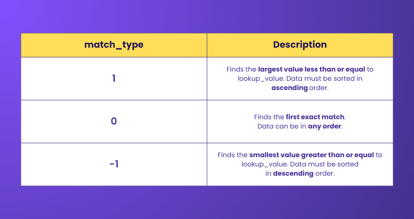
match_type Options Explained

How to Use "MATCH" Function in Excel?

The MATCH function in Excel is used to locate the position of a specific value within a range of cells. Instead of returning the value, it returns the cell’s position number. This is helpful for comparing datasets or setting up dynamic formulas.

Step 1: Open Your Spreadsheet

Open the Excel file that contains your dataset. If you're starting from scratch, create a new sheet and input sample data.

Example: Enter a list of employee names in cells A2 to A6 and prepare to search for one of them.

Step 2: Select the Cell for the MATCH Formula

Click on the cell where you want the position result to appear. This can be anywhere outside your lookup range to keep the data visible.

Example: Select cell C2 to insert the formula.

Step 3: Insert the MATCH Function

Go to the Formulas tab, click Lookup & Reference, and select MATCH from the dropdown list. This opens the function dialog box with three input fields:

a) Lookup_value: The value to search for

b) Lookup_array: The range to search in

c) Match_type: 0 for exact match, 1 for closest match less than value, -1 for closest match greater than value

Example Formula: =MATCH("David", A2:A6, 0)

Step 4: Choose the Match Type

a) 0: Finds the exact match.

b) 1: Finds the largest value less than or equal to the lookup value (data must be sorted in ascending order).

c) -1: Finds the smallest value greater than or equal to the lookup value (data must be sorted in descending order).

Example: If looking for "David", and you want an exact match, choose 0.

Step 5: Verify the Result

After entering the formula, press Enter. Excel will return the position of the value in the specified range.

Example: If “David” is in cell A4, the formula =MATCH("David", A2:A6, 0) will return 3, as A4 is the third cell in the range A2:A6.

Step 6: Handle Mismatches or Errors

If the value is not found and you're using exact match (0), Excel will return #N/A. Double-check spelling, formatting, and ensure the value actually exists in the lookup range.

Example: Searching for “Davd” (misspelled) in the same list will return #N/A.

MATCH Function in Excel - Key pointers

Understanding how to effectively utilise Excel functions can significantly enhance your data analysis skills. Here are a few key points about MATCH Function Excel:

1) When matching text values, the MATCH Function does not make a difference between uppercase and lowercase letters.

2) If the MATCH Function is unable to locate a match for the lookup value, an #N/A error will be generated.

3) The function enables approximate and exact matching along with wildcards (* or?) for partial matches.

4) The location of the first value is returned if the lookup array contains more than one instance of the lookup value.

Become proficient in the top ten Excel shortcuts with our Business Analytics with Excel Course - register today!

Excel VLOOKUP and MATCH

The VLOOKUP function is one of Excel's most popular functions used to search for a value in the first column of a range and return a value in the same row from a specified column. When combined with the MATCH function, users can enhance the flexibility of their lookups.

Using MATCH for Dynamic Column Index: When you use VLOOKUP, you must specify the column index from which to return the value. This is where MATCH comes in handy. Instead of hardcoding the column index, you can use MATCH to dynamically find the correct column based on the header. This is especially useful in tables where columns might be added or rearranged.

Example:

=VLOOKUP (A2, B1:D10, MATCH ("HeaderName", B1:D1, 0), FALSE)

In this formula, MATCH finds the position of "HeaderName" in the first row (B1), and VLOOKUP uses that position as the column index.

Excel HLOOKUP and MATCH

HLOOKUP functions similarly to VLOOKUP but searches for a value in the first row and returns a value from a specified row below it. When combined with MATCH, it provides flexibility in row selection.

Using MATCH for Dynamic Row Index: Much like with VLOOKUP, you can use the MATCH function to dynamically find the row index for HLOOKUP. This is beneficial when working with large datasets or tables where the row structure may vary.

Example:

=HLOOKUP (A2, B1:D10, MATCH ("RowName", A1:A10, 0), FALSE)

Here, MATCH identifies the row of "RowName" in column A, allowing HLOOKUP to return the correct value.

How to match functions in Excel?

In Excel, the MATCH function is used to find the position of a specific value within a row or column. It works with the INDEX function for advanced lookups, helping you locate exact or approximate matches in sorted or unsorted data ranges.

Can VLOOKUP handle multiple matching?

VLOOKUP is designed to return only the first matching value from a range. To handle multiple matches, you need to use advanced formulas like INDEX + SMALL + IF or switch to more flexible functions like FILTER or XLOOKUP in newer Excel versions.

Conclusion

We hope you understand How to Use the Match Function in Excel. The Excel MATCH Function described in this blog is a very handy function for data analysis. Now that you know how it works, keep practicing and exploring more Excel Formulas and Functions!

Excel in advanced MS Excel formulas- sign up for our Microsoft Excel Training today!