What is Dynamic Programming: Types, Advantages and Applications

Key Takeaways

1. Dynamic Programming breaks complex problems into smaller subproblems and reuses their results.

2. Memoisation is top-down, while tabulation follows a bottom-up approach.

3. DP is useful when subproblems overlap and states can be clearly defined.

4. Common applications include optimisation, graphs, sequences and resource allocation.

5. DP can improve efficiency but may require significant memory for large problems.
 

Imagine you are climbing a staircase with 10 steps.

At each move, you can climb either 1 step or 2 steps.

The challenge: How many different ways can you reach the top?

You could calculate every possible route from scratch. Or you could remember what you've already solved:

Step 1 → 1 way

Step 2 → 2 ways

Step 3 → 3 ways

Step 4 → 5 ways

Step 5 → 8 ways

...

Step 10 → 89 ways

Notice the pattern?

Each new answer builds on the results you've already calculated. Instead of repeatedly solving the same smaller problems, you store their answers and reuse them.

This simple idea sits at the heart of Dynamic Programming. But What is Dynamic Programming, how does it work and how can you recognise when a problem needs it? Let's find out.

What is Dynamic Programming?

Dynamic Programming (DP) is an algorithmic problem-solving technique that divides a complex problem into smaller subproblems. Instead of calculating the solution to the same subproblem repeatedly, DP stores previously calculated results and reuses them when needed.

Dynamic Programming is very useful when a problem has overlapping subproblems and optimal substructure. These characteristics allow larger solutions to be constructed efficiently from solutions to smaller problems.

How Does Dynamic Programming Work?

Dynamic Programming generally follows a simple idea:

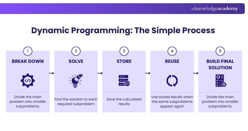
For example, a recursive Fibonacci solution can revisit the same subproblems. Dynamic Programming avoids this repeated work by storing calculated results for reuse.

Key Characteristics of Dynamic Programming

1) Overlapping Subproblems: The same smaller problems appear multiple times while solving the larger problem. DP stores their solutions to avoid repeated computation.

2) Optimal Substructure: The overall problem can be solved by combining optimal solutions from smaller related subproblems.

Types of Dynamic Programming

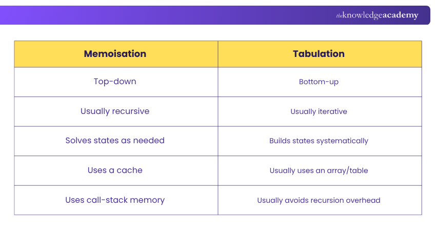
There are two main approaches to Dynamic Programming: memoisation and tabulation. Both store previously calculated results, but they build the solution differently.

1) Top-down Approach (Memoisation)

Memoisation begins with the original problem and recursively breaks it into smaller subproblems. When a subproblem is solved, its result is stored in a cache or suitable data structure.

If the same subproblem appears again, the stored answer is retrieved instead of recalculated.

Key characteristics include:

1) Uses recursion

2) Calculates subproblems when required

3) Stores previously calculated results

4) Can be intuitive when a recursive solution already exists

5) May use additional call-stack memory

Trainer's Pro Tip: If the problem already has a clear recursive structure, start by writing the recurrence relation. You can then add memoisation to remove repeated calculations before considering whether a bottom-up solution would be more efficient.

2) Bottom-up Approach (Tabulation)

Tabulation starts with the smallest known subproblems and gradually builds towards the final solution. Results are commonly stored in an array or table.

Key characteristics include:

1) Usually uses iteration

2) Starts with base cases

3) Builds solutions systematically

4) Avoids recursive call-stack overhead

5) Can sometimes be optimised to use less memory

When to Use Dynamic Programming?

Dynamic Programming is powerful, but it is not suitable for every programming problem. Before using it, check whether the problem has characteristics that make DP useful.

Consider Dynamic Programming when:

1) A recursive or brute-force solution repeatedly performs the same calculations.

2) You can define states that represent smaller versions of the problem.

3) A recurrence or transition connects each state to previously solved states.

4) The number of possible states is manageable enough to compute and store efficiently.

Should You Use Dynamic Programming?

Use this quick decision path:

Can the problem be divided into smaller subproblems?

↓ Yes

Do the same subproblems appear repeatedly?

↓ Yes

Can solutions to smaller subproblems be combined to construct the required overall solution?

↓ Yes

Dynamic Programming may be a suitable approach.

Common Mistake: Do not assume that every recursive problem requires Dynamic Programming. DP is particularly valuable when subproblems overlap and storing their results prevents meaningful repeated work.

How to Solve Dynamic Programming Problems?

Solving a Dynamic Programming problem starts with identifying smaller repeated problems and understanding how their solutions connect. A structured approach helps define the right states, avoid repeated calculations and build the final solution efficiently.

DP Blueprint: Solve Before You Code

Before writing the algorithm, complete this mini blueprint:

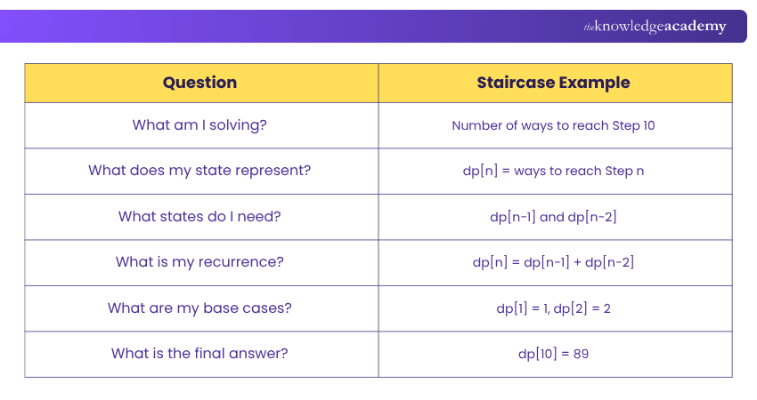
Trainer's Tip: If you cannot clearly define the state, recurrence and base cases, work on the problem logic before writing the code.

1) Define the Problem and State

Start by clearly identifying what needs to be calculated. Then define a state that represents a smaller version of the original problem.

For example, in the staircase problem, dp[n] can represent the number of different ways to reach step n.

2) Create the Recurrence Relation

Determine how the solution to the current state depends on previously solved states.

If you can reach a stair by taking either one or two steps:

dp[n] = dp[n − 1] + dp[n − 2]

This means the number of ways to reach step n equals the ways to reach the previous step plus the ways to reach two steps before it.

3) Define the Base Cases

Set the smallest known solutions so the algorithm has a starting point.

For the staircase example:

dp[1] = 1

dp[2] = 2

These base cases are used to calculate all subsequent states.

Think About It: Before writing any DP code, ask yourself: "What information from an earlier calculation do I need to solve the next state?" The answer can help you identify what your DP state needs to store.

4) Choose Memoisation or Tabulation

Decide how you want to calculate and store the results. Memoisation uses a top-down approach and calculates states when required, while tabulation starts with the base cases and builds the solution from the bottom up.

The best choice depends on the structure of the problem and which states need to be evaluated.

5) Implement the Solution

Build the algorithm using the chosen approach. Each calculated state should be stored so its result can be reused whenever it is needed again.

For example:

dp[3] = dp[2] + dp[1] = 3

The stored value of dp[3] can then help calculate later states.

Can You Complete the DP?

You've defined the states and recurrence. Now, try building the next state yourself.

For the staircase problem:

dp[1] = 1

dp[2] = 2

dp[3] = 3

dp[4] = ?

Using the recurrence:

dp[n] = dp[n−1] + dp[n−2]

Answer: dp[4] = dp[3] + dp[2] = 3 + 2 = 5 

Your turn: What would dp[5] be?

Reveal: dp[5] = dp[4] + dp[3] = 5 + 3 = 8

Continue the same pattern and you eventually reach:

dp[10] = 89

The same recurrence eventually gives dp[10] = 89, bringing us back to the staircase challenge from the introduction.

6) Analyse Time and Space Complexity

Finally, evaluate how the solution performs as the input grows. Check both time complexity and space complexity, then consider whether you can reduce the amount of stored information.

For the staircase problem, you only need the previous two results to calculate the next one. Therefore, a tabulation-based solution can be optimised from O(n) space to O(1) auxiliary space, while maintaining O(n) time.

Gain practical experience with Django's powerful features and functionalities with our Python Django Training – Join today!

Dynamic Programming Algorithms and Examples

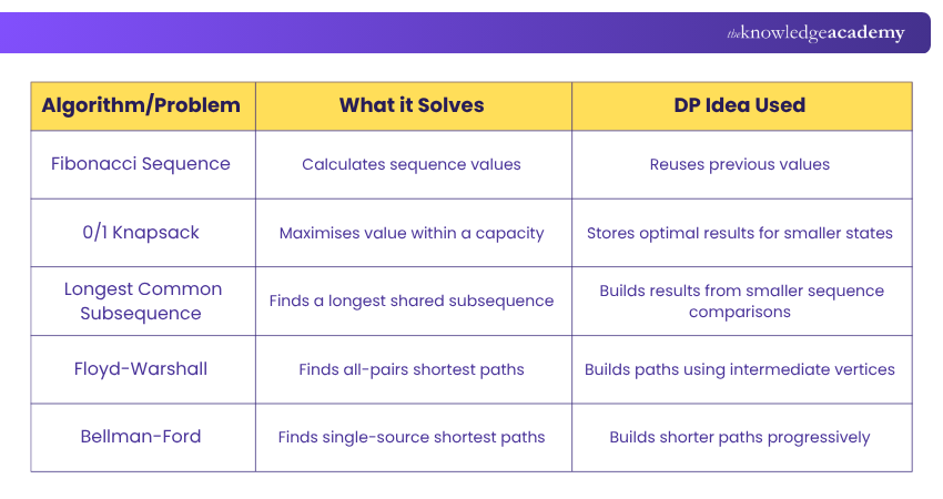
Dynamic Programming is used in many problems where smaller subproblems repeat and their results can contribute to a larger solution. The following examples show how DP can reduce repeated calculations and build solutions systematically:

1) Fibonacci Sequence

The Fibonacci Sequence is one of the simplest ways to understand Dynamic Programming. Each number is calculated using the previous two numbers:

F(n) = F(n−1) + F(n−2)

For example:

F(0) = 0

F(1) = 1

F(2) = 1

F(3) = 2

F(4) = 3

F(5) = 5

A basic recursive approach may calculate the same Fibonacci values many times. Dynamic Programming stores previously calculated values and reuses them, reducing the repeated work. A standard DP solution calculates the sequence in O(n) time.

Quick Insight: Fibonacci is useful for learning DP because the repeated subproblems are easy to see. However, real-world DP problems often involve much more complex states and decisions.

2) 0/1 Knapsack Problem

The 0/1 Knapsack Problem asks you to select items with different weights and values while staying within a fixed weight limit. Each item can either be included once or excluded.

For every item, the algorithm considers:

1) Include it: Add its value and reduce the remaining capacity.

2) Exclude it: Move to the next item without changing the capacity.

Dynamic Programming stores the best result for combinations of items and available capacity. These stored results are then reused to determine the maximum possible value without exceeding the weight limit.

Example: If a knapsack has a capacity of 10 kg, DP can compare item combinations to identify the one with the highest total value without exceeding the limit.

3) Longest Common Subsequence

The Longest Common Subsequence problem finds the longest sequence of elements that appears in two sequences in the same relative order, although the elements do not need to be consecutive.

For example:

Sequence 1: ABCDEF

Sequence 2: ACE

The Longest Common Subsequence is ACE

Dynamic Programming compares prefixes of both sequences and stores the results of smaller comparisons. These results are then used to build the longest common subsequence.

LCS concepts are useful in areas such as sequence comparison and version-difference analysis.

4) Floyd-Warshall Algorithm

The Floyd-Warshall Algorithm uses Dynamic Programming to calculate the shortest distances between all pairs of vertices in a weighted graph.

It progressively checks whether travelling through an intermediate vertex produces a shorter route between two vertices.

Its time complexity is:

O(V³)

where V represents the number of vertices.

Floyd-Warshall can work with negative edge weights, provided shortest paths are well-defined. After the algorithm completes, a negative value on the distance matrix diagonal indicates the presence of a negative-weight cycle.

5) Bellman-Ford Algorithm

The Bellman-Ford Algorithm finds shortest paths from a single source in a weighted graph. It can be viewed as a Dynamic Programming approach because it progressively builds shortest-path estimates using solutions that allow an increasing number of edges. It supports negative edge weights and can also detect reachable negative-weight cycles.

Learn OOP basics like encapsulation, abstraction, and modular design with our Object-oriented Programming (OOPs) Course – Register today!

At a Glance: Where Each Example Fits

Advantages and Limitations of Dynamic Programming

Dynamic Programming can significantly improve suitable algorithms, but it also involves certain trade-offs.

Advantages of Dynamic Programming

1) Reduces Repeated Computation: Previously calculated results can be reused instead of recalculated.

2) Improves Efficiency: DP can substantially reduce the time required by suitable brute-force or recursive solutions.

3) Supports Optimisation Problems: It is widely used for finding minimum costs, maximum values, shortest paths and other optimal results.

4) Encourages Structured Problem-solving: Complex problems can be represented using clearly defined states, recurrence relations and base cases.

5) Supports Diverse Problem Types: DP is useful in graph problems, sequence analysis, resource allocation and other computational tasks.

Limitations of Dynamic Programming

1) Memory Requirements: Storing intermediate states can consume considerable memory for large problems.

2) Difficult State Design: Identifying the correct state and recurrence relation can be challenging.

3) Not Suitable for Every Problem: Problems without useful overlapping subproblems may not benefit from DP.

4) Large State Spaces: Some problems generate so many possible states that even a DP solution becomes expensive.

5) Implementation Complexity: Advanced Dynamic Programming algorithms can be difficult to design, test and debug.

Trainer's Insight: Finding the recurrence relation is often only half the challenge. A strong DP solution also considers the number of states and the amount of work required for each state.

Applications of Dynamic Programming

Dynamic Programming has applications across Computer Science and other fields where complex decisions can be divided into smaller related problems.

1) Graph Algorithms:

DP principles are used in algorithms such as Floyd-Warshall and Bellman-Ford to solve shortest-path problems.

2) Sequence Analysis:

Problems involving sequences can often benefit from DP. Examples include Longest Common Subsequence, edit distance and sequence alignment.

3) Resource Allocation:

Dynamic Programming can help allocate limited resources while maximising value or minimising cost. The Knapsack Problem is a classic example.

4) Computational Biology:

DP is widely used in biological sequence analysis, including DNA and protein sequence alignment.

5)  Artificial Intelligence:

Certain planning, optimisation and sequential decision-making problems can use Dynamic Programming principles.

6) Operations and Scheduling:

DP can be applied to certain scheduling, routing and resource optimisation problems when decisions can be represented as smaller states.

Real-world Insight: Dynamic Programming is most valuable when today's decision affects the options available in later states. By storing the best result for each state, an algorithm can avoid reconsidering the same decision path repeatedly. 

Dynamic Programming vs Greedy Algorithm

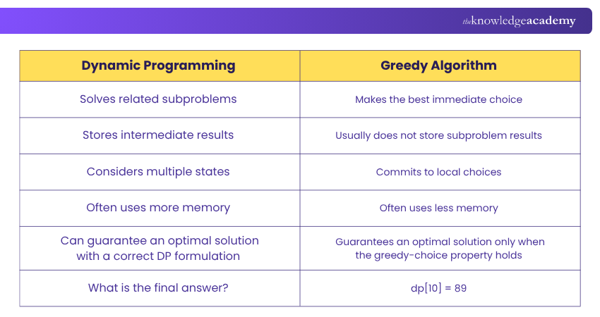
Dynamic Programming and Greedy Algorithms are both used for optimisation problems, but they follow different strategies.

For example, a greedy approach works correctly for problems like finding a minimum spanning tree with Kruskal's Algorithm. However, the 0/1 Knapsack Problem generally requires a different approach, such as Dynamic Programming, to guarantee an optimal solution.

Conclusion

We hope this blog helped you understand What is Dynamic Programming and how it supports efficient problem-solving. From optimisation and graph algorithms to sequence analysis, it offers a structured way to tackle challenging computational tasks. The next time an algorithm repeats its work, ask yourself: Does it really need to solve this again?

Gain hands-on experience working with real-world projects and technologies with our Programming Training – Join now!